When it comes to the Chargers, the talk across the league has revolved around the surprising success around Justin Herbert’s play. What has also shadowed that talk has been the rate at which Chargers have given up double digit leads in 4 straight weeks. Week 4 against Tampa bay they were up 24-7 with 23 seconds left in the second quarter, against New Orleans (week 5) they were up 20-3 with 15 seconds left in the second quarter, up 16-0 with 7:47 left in the 2nd quarter against Jacksonville(week 7) and, the worst one yet, up 24-3 against Denver(week 8) with 6:06 left in the third quarter (week 6 was a bye for the team). Justin Herbert got leads against quarterbacks like Drew Brees and Tom Brady but the defense couldn’t hold the leads for the win. Simultaneously, the Chargers allowed two young 2nd-year quarterbacks to not only regain the lead against their defense but also take the lead with the case of Denver. This type of play is simply unacceptable for a team who was trying to compete for a playoff spot. I will be breaking down the data to see how the defense has played throughout their first 8 games of the season.
I will be using play by play data from the nflfastR R package. Before we dive in i will introduce an important metric which is Expected Points Added (EPA). EPA is based on the down, distance and position on the field and determines how many points you are expected to score after the end of the play. EPA is essentially the difference between the pre-play EPA and the post-play EPA. Below is the first graph of many:
library(tidyverse)
library(nflfastR)
library(ggimage)

def_first<-nfl%>%
  filter((rush_attempt == 1 | pass_attempt == 1) & game_half == 'Half1' & week <= 9)%>%
  group_by(defteam)%>%
  summarize(
    first_mean_epa=mean(epa, na.rm=TRUE)
    )

def_second<-nfl%>%
  filter((rush_attempt == 1 | pass_attempt == 1) & game_half == 'Half2' & week <= 9)%>%
  group_by(defteam)%>%
  summarize(
    second_mean_epa=mean(epa, na.rm=TRUE))

def<-inner_join(def_first, def_second, by=c('defteam'))

def<-inner_join(def, teams_colors_logos,by=c('defteam'='team_abbr'))

ggplot(data=def, aes(x=second_mean_epa, y=first_mean_epa))+
  geom_hline(aes(yintercept = 0), color = 'red', linetype = 'dashed')+
  geom_vline(aes(xintercept = 0), color = 'red', linetype = 'dashed')+
  geom_image(aes(image = team_logo_espn), size = .07)+
  ggtitle('2020 NFL Team Defense ')+
  labs(x = '1st Half EPA Allowed',
       y = '2nd Half EPA Allowed',
       caption = 'Data: nflfastR',
       subtitle = 'week 1-9')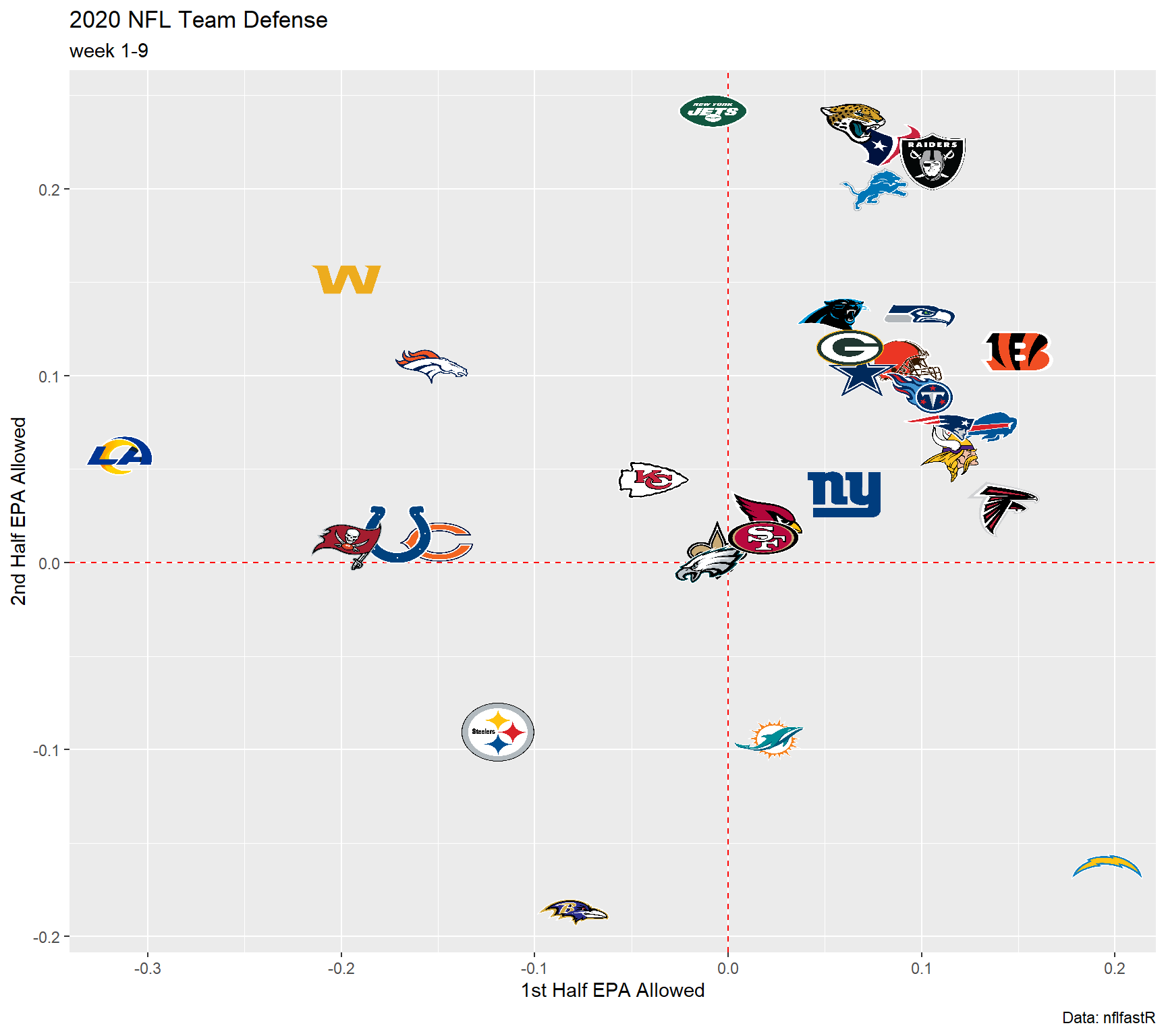
I broke down the defense EPA allowed by half. The Chargers have been excellent in the first half however they do become the worst in the second half. That differnce from first half EPA to second half EPA is the worst in the league. Steelers and Ravens are the only teams with negative average EPA allowed in both halves which indicates how well both defenses play in each half. Lets breakdown the first half:
def_run<-nfl%>%
  filter(rush_attempt == 1 & game_half == 'Half1' & week <= 9)%>%
  group_by(defteam)%>%
  summarize( total_rushes = n(),
    run_mean_epa=mean(epa, na.rm=TRUE))

def_pass<-nfl%>%
  filter(pass_attempt == 1 & game_half == 'Half1' & week <= 9)%>%
  group_by(defteam)%>%
  summarize(total_attempts = n(),
    pass_mean_epa=mean(epa, na.rm=TRUE))

def<-inner_join(def_pass, def_run, by=c('defteam'))

def<-inner_join(def, teams_colors_logos,by=c('defteam'='team_abbr'))

ggplot(data=def, aes(x=run_mean_epa, y=pass_mean_epa))+
  geom_hline(aes(yintercept = 0), color = 'red', linetype = 'dashed')+
  geom_vline(aes(xintercept = 0), color = 'red', linetype = 'dashed')+
  geom_image(aes(image = team_logo_espn), size = .07)+
  ggtitle('NFL Team Defense in the 1st Half')+
  labs(x = 'Run EPA Allowed',
       y = 'Pass EPA Allowed',
       caption = 'Data: nflfastR',
       subtitle = 'week 1-9')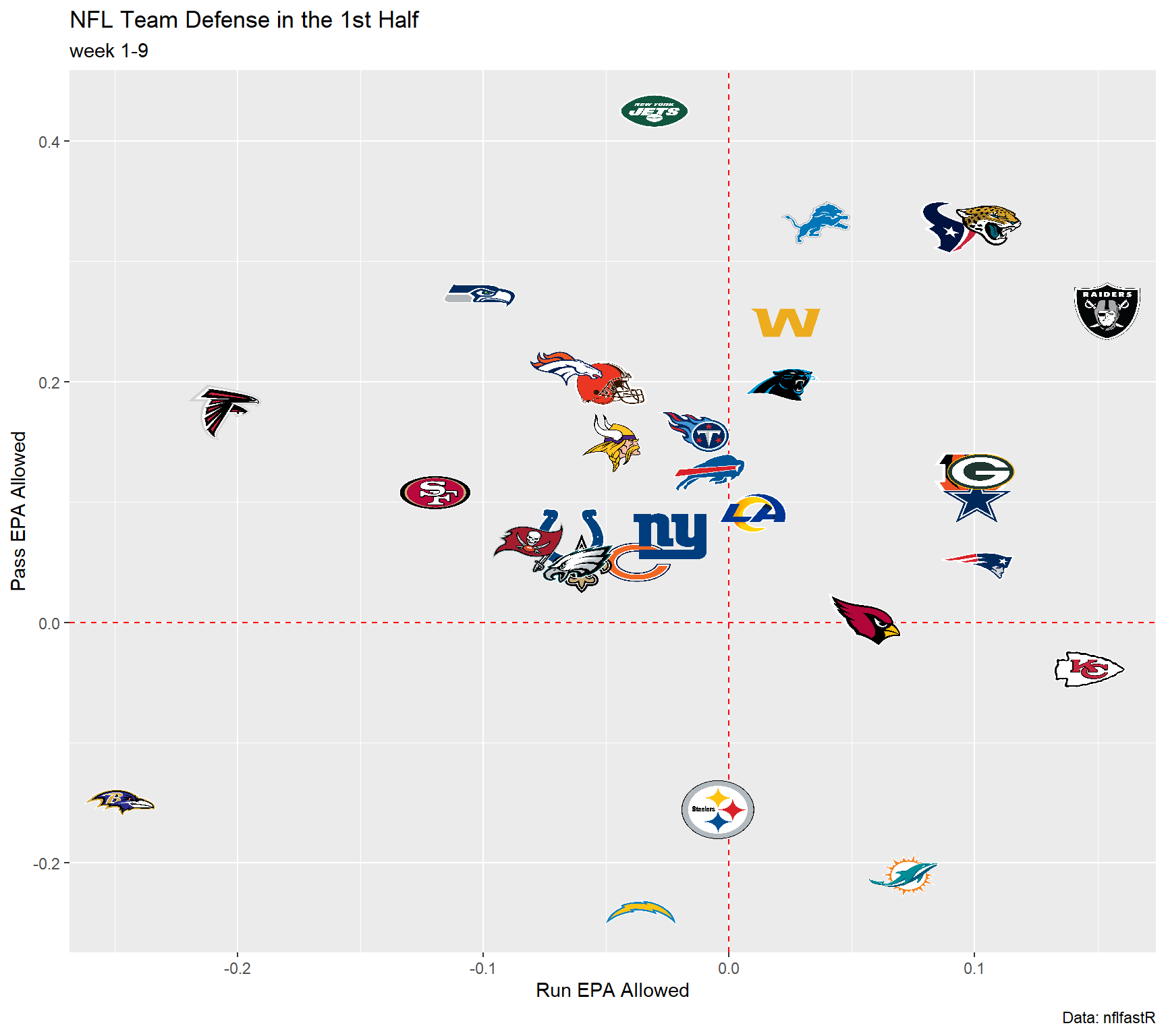
The Chargers make their way in the Ravens and Steelers group. Run defense has been about league average however their pass defense is getting the job done. Next plot is the same as the previous one just from the second half:
def_run<-nfl%>%
  filter(rush_attempt == 1 & game_half == 'Half2' & week <= 9)%>%
  group_by(defteam)%>%
  summarize( total_rushes = n(),
    run_mean_epa=mean(epa, na.rm=TRUE))

def_pass<-nfl%>%
  filter(pass_attempt == 1 & game_half == 'Half2' & week <= 9)%>%
  group_by(defteam)%>%
  summarize(total_attempts = n(),
    pass_mean_epa=mean(epa, na.rm=TRUE))

def<-inner_join(def_pass, def_run, by=c('defteam'))

def<-inner_join(def, teams_colors_logos,by=c('defteam'='team_abbr'))

ggplot(data=def, aes(x=run_mean_epa, y=pass_mean_epa))+
  geom_hline(aes(yintercept = 0), color = 'red', linetype = 'dashed')+
  geom_vline(aes(xintercept = 0), color = 'red', linetype = 'dashed')+
  geom_image(aes(image = team_logo_espn), size = .07)+
  ggtitle('NFL Team Defense in the 2nd Half')+
  labs(x = 'Run EPA Allowed',
       y = 'Pass EPA Allowed',
       caption = 'Data: nflfastR',
       subtitle = 'week 1-9')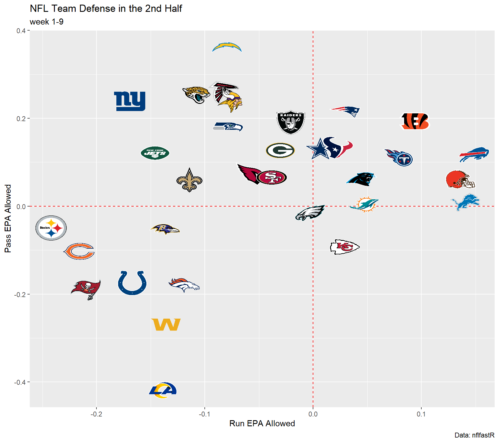
They have essentially flipped the script. While the run defense is just above league average, their second half pass defense goes from first to worst in the league. Their pass defense is what has wrecked their second half defense.
#pass_def <- nfl %>%
#  filter((rush_attempt == 1 | pass_attempt == 1) & week <= 9 & game_half != 'Overtime') %>%
#  group_by(defteam, game_half) %>%
#  summarize(`pass_%`=mean(pass_attempt, na.rm=TRUE)) %>%
#  spread(game_half, `pass_%`) %>%
#  inner_join(teams_colors_logos,by=c('defteam'='team_abbr'))
#
#ggplot(pass_def, aes(x=Half1, y=Half2))+
#  geom_image(aes(image = team_logo_espn), size = .07)+
#  labs(x = 'Defense Mean Run EPA Allowed',
#       y = 'Defense Mean Pass EPA Allowed',
#       caption = 'Data: nflscrapR',
#       subtitle = 'week 1-9')
#
The Chargers have seen 30.125 average plays in the first half while they have seen 28.75 in the second half. They have not seen more plays but what we have seen is a change in location. Average air yards in the first half is about 8.82 yards. Meaning the offense is targeting their receivers on average a little less than 9 yards down the field. In the second half, the average yards targeted dips to 7.85. Likewise offenses have increased their short pass target percentage from 73% in the first half to 82% in the second half. Offenses have also been more explosive(sum of total positive EPA) against the Chargers in the second half. Their second half ranking is 21st while they are 1st (best in the league) in the first half. Chargers have been able to limit the big plays in the first half but they tend to break in the second half.
Situational football
g1 <- nfl %>%
  filter(week <= 9 & game_half != 'Overtime') %>%
  group_by(defteam, game_half)%>%
  summarize(third_con=sum(third_down_converted), third_fail = sum(third_down_failed)) %>%
  mutate(third_attempts=third_con+third_fail,
         third_conversition = third_con/third_attempts) %>%
  select(defteam, game_half, third_conversition) %>%
  spread(game_half, third_conversition) %>%
  inner_join(teams_colors_logos,by=c('defteam'='team_abbr'))%>%
  ggplot(aes(Half1, Half2))+
  geom_image(aes(image=team_logo_espn), size = .07)+
  labs(title = 'NFL Team Defense third down conversation rate',
       subtitle = 'week 1-9',
       caption = 'Data: nflfastR',
        x='1st Half 3rd Down conversition allowed',
        y='2nd Half 3rd Down conversition allowed'
       )


g <- nfl %>%
  filter(week <= 9 &
           game_half != 'Overtime' &
           yardline_100 <= 20 &
           (rush == '1' | pass_attempt == '1')) %>%
  group_by(defteam, game_half)%>%
  summarize(epa = mean(epa, na.rm=TRUE))%>%
  spread(game_half, epa) %>%
  inner_join(teams_colors_logos,by=c('defteam'='team_abbr'))


####
#nfl%>%
#  filter(week <= 9 & game_half != 'Overtime' & (rush == '1' | pass_attempt == '1')) %>%
#  group_by(defteam, game_half)%>%
#  summarize(#epa = mean(epa, na.rm=TRUE),
#            explosivness = sum(epa[epa>0], na.rm=TRUE))%>%
#  spread(game_half, explosivness)%>%
#  inner_join(teams_colors_logos,by=c('defteam'='team_abbr'))%>%
#  ggplot(aes(Half1, Half2))+
#  geom_image(aes(image=team_logo_espn))

g2 <- ggplot()+
  geom_image(data = g, aes(x=Half1, y=Half2, image=team_logo_espn), size = .07)+
  geom_hline(aes(yintercept = 0), color = 'red', linetype = 'dashed')+
  geom_vline(aes(xintercept = 0), color = 'red', linetype = 'dashed')+
  labs(title = 'NFL Red Zone Defense',
       subtitle = 'week 1-9',
       caption = 'Data: nflfastR',
        x='1st Half EPA Allowed',
        y='2nd Half EPA Allowed'
       )

library(patchwork)

g1/g2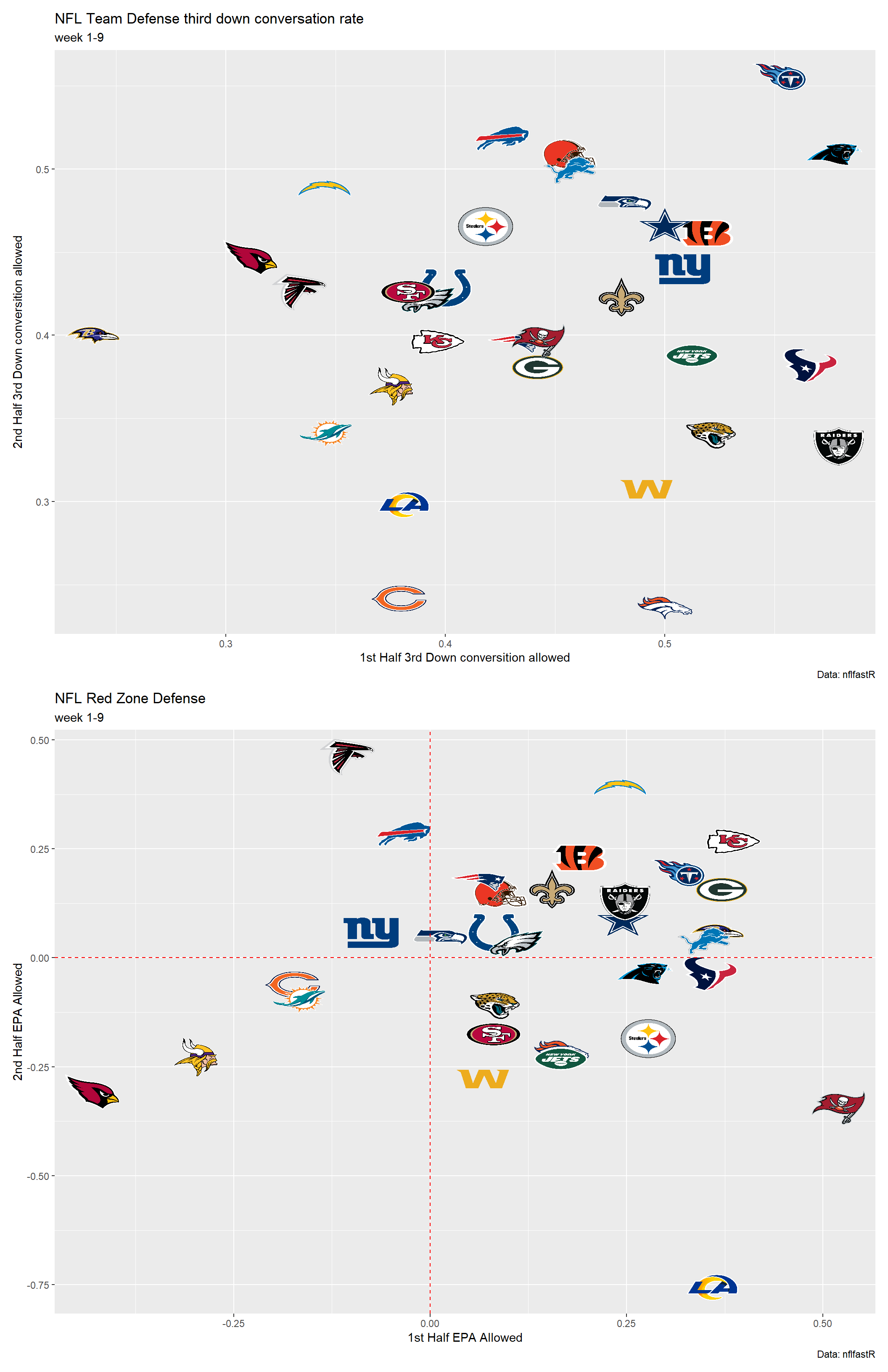
Above i plot each teams third down conversion rate allowed and their Red Zone defense. The Chargers are better in the first half of limiting convestions on third down. Offenses in the first half have on average about 7.2 to the first down line, but in the second half 7.48. Unexpectadly, their average yards to the first down on third down jumps from the first half. The problem for the Chargers is that they haven’t been able to get offenses to third down. If we look at the offenses average yards gained on early downs (1st and 2nd down) in the first half its 4.27 but in the second half is jumps to 6.02. In early downs they are giving up on average more yards in the second half and this prevents them from getting off the field. The Chargers Red zone defense, while mediocre at best in the first half, becomes 2nd worst in the league in the second half.
The Chargers have been unable to make adjustments in the second half of games, and if they have, they haven’t worked. Gus Bradley loves to play Cover 3 and just drop 7 or 8 into coverage and teams know it. What does that mean for the offenses? They are smart and they are going to chip away by attacking the short passing game. While that limits big plays, it doesnt keep them off the field. When the defense is keeping everything in front of them it prevents the secondary from being aggressive and attacking the ball to create turnovers (currently ranked 26th in total tunrovers). Sure they were probably one play away from winning most if not all of those games but they are not put into positions to be aggressive and make a play due to their defensive philosphy.
How bad is this compared to other past teams?
So far, the Chargers defense has been surprisingly bad in the second half compared to how they have played in the first half but how does this compare historically? To find this answer I took the play by play data between 2010 and now and I extracted the rolling 8 game difference in first to second half EPA allowed.The table below includes the top 20 worst teams, the year and the last week included within the 8 week span.
dat <- dat %>% filter(!(season == '2020' & week> 9))

def_first<-dat%>%
    filter((rush_attempt == 1 | pass_attempt == 1) & game_half == 'Half1')%>%
    group_by(defteam, season, week)%>%
    summarize(
        first_mean_epa=mean(epa, na.rm=TRUE)
    )

def_second<-dat%>%
    filter((rush_attempt == 1 | pass_attempt == 1) & game_half == 'Half2')%>%
    group_by(defteam, season, week)%>%
    summarize(
        second_mean_epa=mean(epa, na.rm=TRUE))

def<-inner_join(def_first, def_second, by=c('defteam','season', 'week'))

def<-mutate(def, diff=first_mean_epa - second_mean_epa)


test2 <- def %>%
    arrange(defteam, season, week) %>%
    group_by(defteam) %>%
    mutate(eight_week_mean = zoo::rollmean(diff, 8, align = 'right', fill = NA)) %>%
    ungroup()

library(gt)

test2 %>%
  select(defteam, season, week, eight_week_mean) %>%
  arrange(eight_week_mean) %>%
  mutate(defteam=tolower(defteam))%>%
  top_n(-20)%>%
  gt() %>%
  text_transform(locations = cells_body(vars(defteam)),
                 fn = function(x) web_image(url = paste0('https://a.espncdn.com/i/teamlogos/nfl/500/',x, '.png'))) %>%
  cols_label(
    defteam = "Team",
    season = "Season",
    week = "Week",
    eight_week_mean = '8 week diffence in EPA'
  )%>%
  tab_header(
    title = md("**NFL Teams Worst 8 game difference in first to Second half defense EPA**"),
    subtitle = md("*NOTE: Playoffs are not included and the 8 game difference does rollover from the previous season*")
)| NFL Teams Worst 8 game difference in first to Second half defense EPA | |||
|---|---|---|---|
| NOTE: Playoffs are not included and the 8 game difference does rollover from the previous season | |||
| Team | Season | Week | 8 week diffence in EPA |
 |
2020 | 9 | -0.3360044 |
|
2020 | 8 | -0.3274325 |
 |
2017 | 2 | -0.3181187 |
|
2017 | 3 | -0.3048038 |
 |
2017 | 3 | -0.3045694 |
|
2017 | 4 | -0.2905659 |
 |
2020 | 3 | -0.2865451 |
|
2017 | 4 | -0.2792833 |
 |
2018 | 16 | -0.2792074 |
|
2017 | 6 | -0.2779420 |
|
2018 | 14 | -0.2764476 |
|
2018 | 15 | -0.2743025 |
|
2018 | 17 | -0.2737844 |
 |
2016 | 11 | -0.2727742 |
 |
2019 | 4 | -0.2721691 |
 |
2018 | 9 | -0.2669310 |
 |
2015 | 9 | -0.2658105 |
|
2017 | 1 | -0.2651233 |
|
2020 | 5 | -0.2636887 |
|
2016 | 6 | -0.2636884 |
The 2020 Chargers take the top two spots. That difference in first to second half defense has been historically bad. While you can blame Gus Bradley’s scheme or the players, there was a level of randomness for this defense this year. Now this stretch could not be carried over into the rest of this year or even potentially next year. Just because the Chargers have played historically bad in the beginning of this year, it doesnt mean they will continue to play historically bad. They have the players to play well, evident in how they play in the first half,but its just whether they can overcome the adversity they have been hit with and play with confidence.